Perceptron
Introduction
The Perceptron Learning Algorithm (PLA) is a supervised learning algorithm widely employed for binary classification tasks. Its primary objective is to determine a decision boundary that effectively separates the two classes in the dataset. This algorithm belongs to the class of discriminative classification methods as it focuses on modeling the boundary between classes instead of characterizing the underlying probability distribution of each class.
Let \(D=\{(\mathbf{x}_1, y_1), \ldots, (\mathbf{x}_n,y_n)\}\) represent the dataset, where \(\mathbf{x}_i \in \mathbb{R}^d\) and \(y_i \in \{0, 1\}\).
The algorithm is founded on the following assumptions:
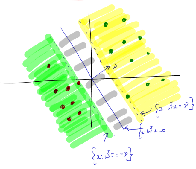
- \(P(y=1|\mathbf{x}) = 1\) if \(\mathbf{w}^\mathbf{T}\mathbf{x}\geq0\), otherwise \(P(y=1|\mathbf{x}) = 0\).
- Linear Separability Assumption: The Linear Separability Assumption is a fundamental assumption made in various machine learning algorithms, including the Perceptron Learning Algorithm. It posits that the classes to be classified can be accurately separated by a linear decision boundary. In other words, there exists a hyperplane in the feature space that can effectively segregate the data points of the two classes.
The objective function is defined as follows:
\[ \min _{h \in \mathcal{H}} \sum _{i=1} ^n \mathbb{1}\left ( h(\mathbf{x}_i) \neq y_i \right ) \]
Even if \(\mathcal{H}\) accounts only for the Linear Hypotheses, this problem is generally considered NP-Hard.
Under the Linear Separability Assumption, assuming the existence of \(\mathbf{w} \in \mathbb{R}^d\) such that \(\text{sign}(\mathbf{w}^\mathbf{T}\mathbf{x}_i)=y_i\) holds for all \(i \in \{1, 2, \ldots, n\}\), the PLA solves the convergence problem using an iterative algorithm. The algorithm proceeds as follows:
- Initialize \(\mathbf{w}^0 = \mathbf{0} \in \mathbb{R}^d\)
- Until Convergence:
- Select a \((\mathbf{x}_i, y_i)\) pair from the dataset
- If \(\text{sign}(\mathbf{w}^\mathbf{T}\mathbf{x}_i)==y_i\)
- Do nothing
- Else
- Update the weight vector: \(\mathbf{w}^{(t+1)} = \mathbf{w}^t + \mathbf{x}_iy_i\)
- End
Analysis of the Update Rule
For a given training example \((\mathbf{x}, y)\), where \(\mathbf{x}\) represents the input and \(y\) represents the correct output (either \(1\) or \(-1\)), the perceptron algorithm updates the weight vector \(\mathbf{w}\) according to the following rules:
- If the perceptron’s prediction on \(\mathbf{x}\) is correct (i.e., \(\text{sign}(\mathbf{w}^\mathbf{T}\mathbf{x}_i)==y_i\)), no update is performed.
- If the perceptron’s prediction on \(\mathbf{x}\) is incorrect (i.e., \(\text{sign}(\mathbf{w}^\mathbf{T}\mathbf{x}_i)\neq y_i\)), the weights are updated by adding the product of the input vector and the correct output to the current weight vector: \(\mathbf{w}^{(t+1)} = \mathbf{w}^t + \mathbf{x}_iy_i\).
- It is important to note that the update occurs solely in response to the current data point. Consequently, data points that were previously classified correctly may not be classified similarly in future iterations.
This update rule effectively adjusts the decision boundary in the direction of correct classification for the misclassified example. The algorithm is guaranteed to converge to a linearly separable solution if the data is indeed linearly separable. However, if the data is not linearly separable, the perceptron algorithm may not converge to a solution.
Further Assumptions
We introduce three additional assumptions:
- Linear Separability with \(\gamma\)-Margin: A dataset \(D=\{(\mathbf{x}_1, y_1), \ldots, (\mathbf{x}_n,y_n)\}\) is considered linearly separable with a \(\gamma\)-margin if there exists \(\mathbf{w}^* \in \mathbb{R}^d\) such that \((\mathbf{w}^{*T}\mathbf{x}_i)y_i\geq\gamma\) holds for all \(i\), where \(\gamma>0\).
- Radius Assumption: Let \(R>0 \in \mathbb{R}\) be a constant such that \(\forall i \in D\), \(||\mathbf{x}_i||\leq R\). In other words, \(R\) denotes the length of the data point farthest from the center.
- Normal Length for \(\mathbf{w}^*\): Assume that \(\mathbf{w}^*\) has unit length.
Proof of Convergence of Perceptron Algorithm
We denote the current mistake number as \(l\). Based on our previous findings, we can observe the following:
\[\begin{align*} \mathbf{w}^{l+1} &= \mathbf{w}^l + \mathbf{x}y \\ ||\mathbf{w}^{l+1}||^2&=||\mathbf{w}^l + \mathbf{x}y||^2 \\ &=(\mathbf{w}^l + \mathbf{x}y)^T(\mathbf{w}^l + \mathbf{x}y) \\ &=||\mathbf{w}^l||^2 + 2(\mathbf{w}^{lT}\mathbf{x})y+ ||\mathbf{x}||^2y^2 \\ \therefore ||\mathbf{w}^{l+1}||^2&\leq ||\mathbf{w}^l||^2 + R^2 \\ &\leq (||\mathbf{w}^{l-1}||^2 + R^2) + R^2 \\ &\leq ||\mathbf{w}^0||^2 + lR^2 \\ \therefore ||\mathbf{w}^{l+1}||^2&\leq lR^2 \hspace{6em} \ldots[1] \end{align*}\]
Furthermore, we have:
\[\begin{align*} \mathbf{w}^{l+1} &= \mathbf{w}^l + \mathbf{x}y \\ (\mathbf{w}^{l+1})^T\mathbf{w}^* &= (\mathbf{w}^l + \mathbf{x}y)^T\mathbf{w}^* \\ &= \mathbf{w}^{lT}\mathbf{w}^* + (\mathbf{w}^{*T}\mathbf{x})y \\ \therefore (\mathbf{w}^{l+1})^T\mathbf{w}^* &\geq \mathbf{w}^{lT}\mathbf{w}^* + \gamma \\ &\geq (\mathbf{w}^{l-1T}\mathbf{w}^* + \gamma) + \gamma \\ &\geq \mathbf{w}^{0T}\mathbf{w}^* + l\gamma \\ \therefore (\mathbf{w}^{l+1})^T\mathbf{w}^* &\geq l\gamma \\ ((\mathbf{w}^{l+1})^T\mathbf{w}^*)^2 &\geq l^2\gamma^2 \\ ||\mathbf{w}^{l+1}||^2||\mathbf{w}^*||^2 &\geq l^2\gamma^2 \hspace{0.5em}\ldots\text{Using the Cauchy-Schwarz inequality}\\ \therefore ||\mathbf{w}^{l+1}||^2 &\geq l^2\gamma^2 \hspace{6em} \ldots[2] \end{align*}\]
Combining equations \([1]\) and \([2]\), we obtain:
\[\begin{align*} l^2\gamma^2 &\leq ||\mathbf{w}^{l+1}||^2 \leq lR^2 \\ l^2\gamma^2 &\leq lR^2 \\ \therefore l &\leq \frac{R^2}{\gamma^2} \end{align*}\]
Consequently, the above equation establishes an upper bound on the number of mistakes for datasets conforming to the Linear Separability with \(\gamma\)-Margin property and having a finite radius \(R\). This result demonstrates the convergence of the perceptron algorithm.