Logistic regression
Sigmoid Function
Until now, we have utilized the \(\text{sign}\) function to determine the class for the output. However, what if we also wish to obtain the probabilities associated with these outputs?
Let \(z=\mathbf{w}^\mathbf{T}\mathbf{x}\), where \(z \in \mathbb{R}\). How can we map \([-\infty, \infty]\rightarrow[0,1]\)? To address this, we introduce the Sigmoid Function, defined as follows:
\[ g(z) = \frac{1}{1+e^{-z}} \]
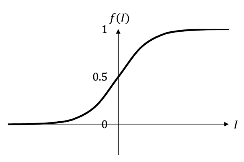
The sigmoid function is commonly employed in machine learning as an activation function for neural networks. It exhibits an S-shaped curve, making it well-suited for modeling processes with a threshold or saturation point, such as logistic growth or binary classification problems.
For large positive input values, the sigmoid function approaches 1, while for large negative input values, it approaches 0. When the input value is 0, the sigmoid function output is exactly 0.5.
The term “sigmoid” is derived from the Greek word “sigmoides,” meaning “shaped like the letter sigma” (\(\Sigma\)). The sigmoid function’s characteristic S-shaped curve resembles the shape of the letter sigma, which likely influenced the function’s name.
Logistic Regression
Logistic regression is a statistical method used to analyze and model the relationship between a binary (two-valued) dependent variable and one or more independent variables. The independent variables can be either continuous or categorical. The main objective of logistic regression is to estimate the probability that the dependent variable belongs to one of the two possible values, given the independent variable values.
In logistic regression, the dependent variable is modeled as a function of the independent variables using a logistic (sigmoid) function. This function generates an S-shaped curve ranging between 0 and 1. By transforming the output of a linear combination of the independent variables using the logistic function, logistic regression provides a probability estimate that can be used for classifying new observations.
Let \(D=\{(\mathbf{x}_1, y_1), \ldots, (\mathbf{x}_n,y_n)\}\) denote the dataset, where \(\mathbf{x}_i \in \mathbb{R}^d\) and \(y_i \in \{0, 1\}\).
We know that:
\[ P(y=1|\mathbf{x}) = g(\mathbf{w}^\mathbf{T}\mathbf{x}_i) = \frac{1}{1+e^{-\mathbf{w}^\mathbf{T}\mathbf{x}}} \]
Using the maximum likelihood approach, we can derive the following expression:
\[\begin{align*} \mathcal{L}(\mathbf{w};\text{Data}) &= \prod _{i=1} ^{n} (g(\mathbf{w}^\mathbf{T}\mathbf{x}_i))^{y_i}(1- g(\mathbf{w}^\mathbf{T}\mathbf{x}_i))^{1-y_i} \\ \log(\mathcal{L}(\mathbf{w};\text{Data})) &= \sum _{i=1} ^{n} y_i\log(g(\mathbf{w}^\mathbf{T}\mathbf{x}_i))+(1-y_i)\log(1- g(\mathbf{w}^\mathbf{T}\mathbf{x}_i)) \\ &= \sum _{i=1} ^{n} y_i\log\left(\frac{1}{1+e^{-\mathbf{w}^\mathbf{T}\mathbf{x}_i}}\right)+(1-y_i)\log\left(\frac{e^{-\mathbf{w}^\mathbf{T}\mathbf{x}_i}}{1+e^{-\mathbf{w}^\mathbf{T}\mathbf{x}_i}}\right) \\ &= \sum _{i=1} ^{n} \left [ (1-y_i)(-\mathbf{w}^\mathbf{T}\mathbf{x}_i) - \log(1+e^{-\mathbf{w}^\mathbf{T}\mathbf{x}_i}) \right ] \end{align*}\]
Therefore, our objective, which involves maximizing the log-likelihood function, can be formulated as follows:
\[ \max _{\mathbf{w}}\sum _{i=1} ^{n} \left [ (1-y_i)(-\mathbf{w}^\mathbf{T}\mathbf{x}_i) - \log(1+e^{-\mathbf{w}^\mathbf{T}\mathbf{x}_i}) \right ] \]
However, a closed-form solution for this problem does not exist. Therefore, we resort to using gradient descent for convergence.
The gradient of the log-likelihood function is computed as follows:
\[\begin{align*} \nabla \log(\mathcal{L}(\mathbf{w};\text{Data})) &= \sum _{i=1} ^{n} \left [ (1-y_i)(-\mathbf{x}_i) - \left( \frac{e^{-\mathbf{w}^\mathbf{T}\mathbf{x}_i}}{1+e^{-\mathbf{w}^\mathbf{T}\mathbf{x}_i}} \right ) (-\mathbf{x}_i) \right ] \\ &= \sum _{i=1} ^{n} \left [ -\mathbf{x}_i + \mathbf{x}_iy_i + \mathbf{x}_i \left( \frac{e^{-\mathbf{w}^\mathbf{T}\mathbf{x}_i}}{1+e^{-\mathbf{w}^\mathbf{T}\mathbf{x}_i}} \right ) \right ] \\ &= \sum _{i=1} ^{n} \left [ \mathbf{x}_iy_i - \mathbf{x}_i \left( \frac{1}{1+e^{-\mathbf{w}^\mathbf{T}\mathbf{x}_i}} \right ) \right ] \\ \nabla \log(\mathcal{L}(\mathbf{w};\text{Data})) &= \sum _{i=1} ^{n} \left [ \mathbf{x}_i \left(y_i - \frac{1}{1+e^{-\mathbf{w}^\mathbf{T}\mathbf{x}_i}} \right ) \right ] \end{align*}\]
Utilizing the gradient descent update rule, we obtain:
\[\begin{align*} \mathbf{w}_{t+1} &= \mathbf{w}_t + \eta_t\nabla \log(\mathcal{L}(\mathbf{w};\text{Data})) \\ &= \mathbf{w}_t + \eta_t \left ( \sum _{i=1} ^{n} \mathbf{x}_i \left(y_i - \frac{1}{1+e^{-\mathbf{w}^\mathbf{T}\mathbf{x}_i}} \right ) \right ) \end{align*}\]
Kernel and Regularized Versions
It is possible to argue that \(\mathbf{w}^*=\displaystyle\sum _{i=1} ^{n}\alpha_i\mathbf{x}_i\), thereby allowing for kernelization. For additional information, please refer to this link.
The regularized version of logistic regression can be expressed as follows:
\[ \min _{\mathbf{w}}\sum _{i=1} ^{n} \left [ \log(1+e^{-\mathbf{w}^\mathbf{T}\mathbf{x}_i}) + \mathbf{w}^\mathbf{T}\mathbf{x}_i(1-y_i) \right ] + \frac{\lambda}{2}||\mathbf{w}||^2 \]
Here, \(\frac{\lambda}{2}||\mathbf{w}||^2\) serves as the regularizer, and \(\lambda\) is determined through cross-validation.