K-nearest neighbors (KNN)
Introduction to Binary Classification
Binary classification is a fundamental task in machine learning, commonly employed in various domains such as computer vision, natural language processing, and bioinformatics. Its objective is to assign objects into one of two categories based on their features.
Consider a dataset \(\{\mathbf{x}_1, \ldots, \mathbf{x}_n\}\), where \(\mathbf{x}_i \in \mathbb{R}^d\), and let \(\{y_1, \ldots, y_n\}\) be the corresponding labels, where \(y_i \in \{0, 1\}\). The goal is to find a function \(h: \mathbb{R}^d \rightarrow \{0, 1\}\) that accurately predicts the labels.
To assess the performance of the classification function, a loss measure is employed. The loss function is defined as follows:
\[ \text{loss}(h) = \frac{1}{n} \sum ^n _{i=1}\mathbb{1}\left ( h(\mathbf{x}_i) \ne y_i \right ) \]
Let \(\mathcal{H}_{\text{linear}}\) denote the solution space for the linear mapping:
\[ \mathcal{H}_{\text{linear}}=\left\{\mathbf{h}_w: \mathbb{R}^d \rightarrow \{1, 0\} \hspace{0.5em} \text{s.t.} \hspace{0.5em} \mathbf{h}_w(\mathbf{x}) = \text{sign}(\mathbf{w}^T\mathbf{x}) \hspace{0.5em} \forall \mathbf{w} \in \mathbb{R}^d \right\} \]
Hence, the objective function can be expressed as:
\[ \min_{h \in \mathcal{H}_{\text{linear}}} \sum_{i=1}^n \mathbb{1}\left ( h(\mathbf{x}_i) \ne y_i \right ) \]
However, it is important to note that this objective function presents an NP-Hard problem, making it challenging to find optimal and sufficient parameters. Therefore, improved implementations are required to address this complexity and achieve satisfactory results.
Linear Classifier
Can linear regression be used to solve the binary classification problem? Let’s examine the proposed algorithm:
\[ \{(\mathbf{x}_1, y_1), \ldots, (\mathbf{x}_n,y_n)\} \xrightarrow[Regression]{Linear} \mathbf{w} \in \mathbb{R}^d \rightarrow \mathbf{h}_\mathbf{w}: \mathbb{R}^d \rightarrow \{1, 0\} \]
However, employing linear regression for classification poses an issue. Consider the following diagram:
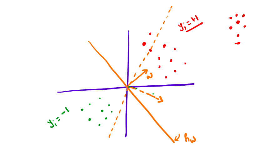
Upon closer examination, it becomes evident that linear regression-based classification not only separates the two categories based on their respective sides but also considers their positions. As a consequence, the classification boundary may shift with respect to the outliers in the dataset. Hence, this approach is not suitable for binary classification.
K-Nearest Neighbors Algorithm
The K-Nearest Neighbors (K-NN) algorithm is a widely-used non-parametric method utilized for both classification and regression tasks in machine learning. It operates by identifying the K-nearest data points to the target object and classifying or regressing the target object based on the majority of its nearest neighbors.
The algorithm follows these steps:
- Given a test sample \(\mathbf{x}_{\text{test}}\), find the \(k\) closest points in the training set, denoted as \(\{\mathbf{x}_1^*, \mathbf{x}_2^*, \ldots, \mathbf{x}_k^*\}\).
- Predict the label of the test sample as \(y_{\text{test}} = \text{majority}(y_1^*, y_2^*, \ldots, y_k^*)\).
The following diagrams illustrate the impact of the value of \(k\) on the classification:
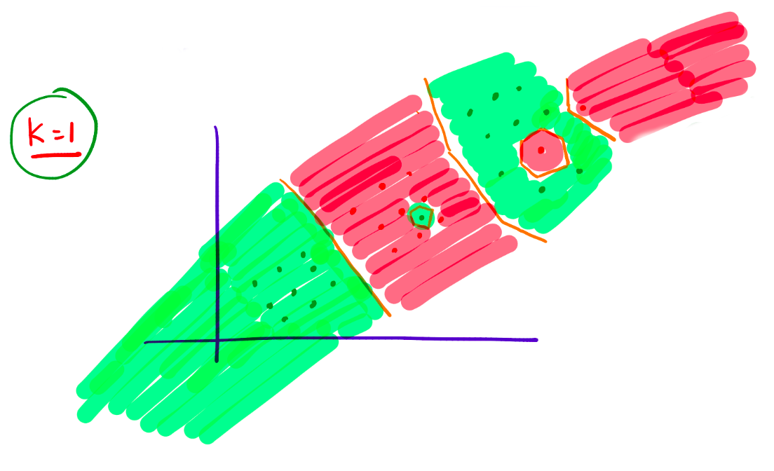 \[
\text{When }k=1\text{, the classification is highly sensitive to outliers.}
\]
\[
\text{When }k=1\text{, the classification is highly sensitive to outliers.}
\] 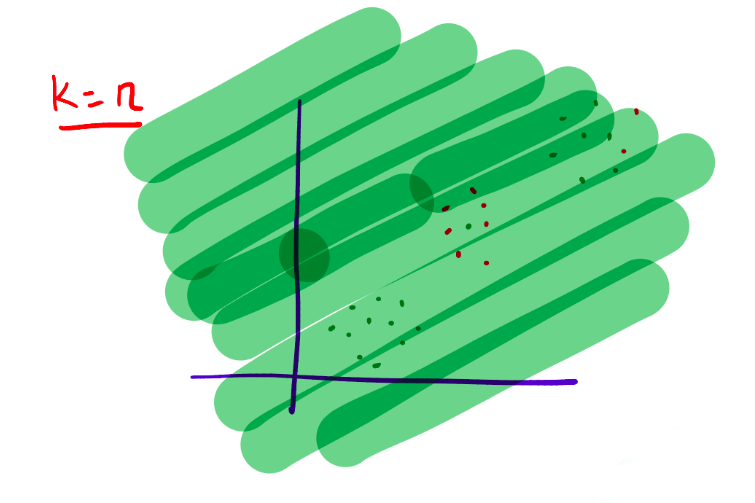 \[
\text{When }k=n\text{, the classification becomes overly smooth.}
\]
\[
\text{When }k=n\text{, the classification becomes overly smooth.}
\] 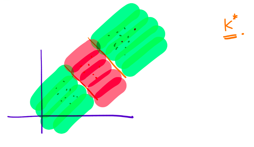 \[
\text{When }k=k^*\text{, the classification achieves a balanced result.}
\]
\[
\text{When }k=k^*\text{, the classification achieves a balanced result.}
\]
The choice of \(k\) is typically determined through cross-validation, treating \(k\) as a hyperparameter. Smaller values of \(k\) lead to more complex classifications.
Issues with K-NN
The K-NN algorithm suffers from several limitations:
- The choice of distance function can yield different results. The Euclidean distance, commonly used, might not always be the best fit for all scenarios.
- Computationally, the algorithm can be demanding. When making predictions for a single test data point, the distances between that data point and all training points must be calculated and sorted. Consequently, the algorithm has a complexity of \(O(n \log(n))\), where \(n\) represents the size of the dataset.
- The algorithm does not learn a model but instead relies on the training dataset for making predictions.