Principal Component Analysis
Representation Learning
Representation learning is a fundamental sub-field of machine learning that is concerned with acquiring meaningful and compact representations of intricate data, facilitating various tasks such as dimensionality reduction, clustering, and classification.
Let us consider a dataset \(\{\mathbf{x}_1, \mathbf{x}_2, \ldots, \mathbf{x}_n\}\), where each \(\mathbf{x}_i \in \mathbb{R}^{d}\). The objective is to find a representation that minimizes the reconstruction error.
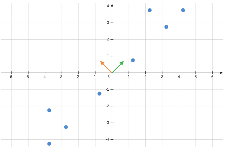
We can start by seeking the best linear representation of the dataset, denoted by \(\mathbf{w}\), subject to the constraint \(||\mathbf{w}||=1\).
The representation is given by, \[\begin{align*} \frac{(\mathbf{x}_i^T\mathbf{w})}{\mathbf{w}^T\mathbf{w}}&\mathbf{w} \\ \text{However, }||\mathbf{w}||&=1\\ \therefore \text{ Projection } &= (\mathbf{x}_i^T\mathbf{w})\mathbf{w} \end{align*}\]
The reconstruction error is computed as follows, \[ \text{Reconstruction Error}(f(\mathbf{w})) = \frac{1}{n} \sum _{i=1} ^{n} || \mathbf{x}_i - (\mathbf{x}_i^T\mathbf{w})\mathbf{w} || ^ 2 \] where \(\mathbf{x}_i - (\mathbf{x}_i^T\mathbf{w})\mathbf{w}\) is termed the residue and can be represented as \(\mathbf{x}'\).
The primary aim is to minimize the reconstruction error, leading to the following optimization formulation: \[\begin{align*} \min _{\mathbf{w} \in ||\mathbf{w}|| = 1} f(\mathbf{w}) &= \frac{1}{n} \sum _{i=1} ^{n} -(\mathbf{x}_i^T\mathbf{w})^2 \\ \therefore \max _{\mathbf{w} \in ||\mathbf{w}|| = 1} f(\mathbf{w}) &= \frac{1}{n} \sum _{i=1} ^{n} (\mathbf{x}_i^T\mathbf{w})^2 \\ &= \mathbf{w}^T(\frac{1}{n} \sum _{i=1} ^{n} \mathbf{x}_i\mathbf{x}_i^T)\mathbf{w} \\ \max _{\mathbf{w} \in ||\mathbf{w}|| = 1} f(\mathbf{w}) &= \mathbf{w}^T\mathbf{C}\mathbf{w} \end{align*}\] where \(\mathbf{C}=\displaystyle \frac{1}{n} \displaystyle \sum _{i=1} ^{n} \mathbf{x}_i\mathbf{x}_i^T\) represents the Covariance Matrix, and \(\mathbf{C} \in \mathbb{R}^{d \times d}\).
Notably, the eigenvector \(\mathbf{w}\) corresponding to the largest eigenvalue \(\lambda\) of \(\mathbf{C}\) becomes the sought-after solution for the representation. This \(\mathbf{w}\) is often referred to as the First Principal Component of the dataset.
Potential Algorithm
Based on the above concepts, we can outline the following algorithm for representation learning:
Given a dataset \(\{\mathbf{x}_1, \mathbf{x}_2, \ldots, \mathbf{x}_n\}\) where \(\mathbf{x}_i \in \mathbb{R}^{d}\),
Center the dataset: \[ \mathbf{\mu} = \frac{1}{n} \sum _{i=1} ^{n} \mathbf{x}_i \] \[ \mathbf{x}_i = \mathbf{x}_i - \mathbf{\mu} \hspace{2em} \forall i \]
Find the best representation \(\mathbf{w} \in \mathbb{R}^d\) with \(||\mathbf{w}|| = 1\).
Update the dataset with the representation: \[ \mathbf{x}_i = \mathbf{x}_i - (\mathbf{x}_i^T\mathbf{w})\mathbf{w} \hspace{1em} \forall i \]
Repeat steps 2 and 3 until the residues become zero, resulting in \(\mathbf{w}_2, \mathbf{w}_3, \ldots, \mathbf{w}_d\).
The question arises: Is this the most effective approach, and how many \(\mathbf{w}\) do we need to achieve optimal compression?
Principal Component Analysis
Principal Component Analysis (PCA) is a powerful technique employed to reduce the dimensionality of a dataset by identifying its most important features, known as principal components, which explain the maximum variance present in the data. PCA achieves this by transforming the original dataset into a new set of uncorrelated variables, ordered by their significance in explaining the variance. This process is valuable for visualizing high-dimensional data and preprocessing it before conducting machine learning tasks.
Following the potential algorithm mentioned earlier and utilizing the set of eigenvectors \(\{\mathbf{w}_1, \mathbf{w}_2, \ldots, \mathbf{w}_d\}\), we can express each data point \(\mathbf{x}_i\) as a linear combination of the projections on these eigenvectors: \[ \forall i \hspace{1em} \mathbf{x}_i - ((\mathbf{x}_i^T\mathbf{w}_1)\mathbf{w}_1 + (\mathbf{x}_i^T\mathbf{w}_2)\mathbf{w}_2 + \ldots +(\mathbf{x}_i^T\mathbf{w}_d)\mathbf{w}_d) = 0 \] \[ \therefore \mathbf{x}_i = (\mathbf{x}_i^T\mathbf{w}_1)\mathbf{w}_1 + (\mathbf{x}_i^T\mathbf{w}_2)\mathbf{w}_2 + \ldots +(\mathbf{x}_i^T\mathbf{w}_d)\mathbf{w}_d \]
From the above equation, we observe that we can represent the data using constants \(\{\mathbf{x}_i^T\mathbf{w}_1, \mathbf{x}_i^T\mathbf{w}_2, \ldots, \mathbf{x}_i^T\mathbf{w}_d\}\) along with vectors \(\{\mathbf{w}_1, \mathbf{w}_2, \ldots, \mathbf{w}_d\}\).
Thus, a dataset initially represented as \(d \times n\) can now be compressed to \(d (d + n)\) elements, which might seem suboptimal at first glance.
However, if the data resides in a lower-dimensional subspace, the residues can be reduced to zero without requiring all \(d\) principal components. Suppose the data can be adequately represented using only \(k\) principal components, where \(k \ll d\). In that case, the data can be efficiently compressed from \(d \times n\) to \(k(d + n)\).
Approximate Representation
The question arises: If the data can be approximately represented by a lower-dimensional subspace, would it suffice to use only those \(k\) projections? Additionally, how much variance should be covered?
Let us consider a centered dataset \(\{\mathbf{x}_1, \mathbf{x}_2, \ldots, \mathbf{x}_n\}\) where \(\mathbf{x}_i \in \mathbb{R}^{d}\). Let \(\mathbf{C}\) represent its covariance matrix, and \(\{\lambda_1, \lambda_2, \ldots, \lambda_d \}\) be the corresponding eigenvalues, which are non-negative due to the positive semi-definiteness of the covariance matrix. These eigenvalues are arranged in descending order, with \(\{\mathbf{w}_1, \mathbf{w}_2, \ldots, \mathbf{w}_d \}\) as their corresponding eigenvectors of unit length.
The eigen equation for the covariance matrix can be expressed as follows: \[\begin{align*} \mathbf{C}\mathbf{w} &= \lambda \mathbf{w} \\ \mathbf{w}^T\mathbf{C}\mathbf{w} &= \mathbf{w}^T\lambda \mathbf{w}\\ \therefore \lambda &= \mathbf{w}^T\mathbf{C}\mathbf{w} \hspace{2em} \{\mathbf{w}^T\mathbf{w} = 1\} \\ \lambda &= \frac{1}{n} \sum _{i=1} ^{n} (\mathbf{x}_i^T\mathbf{w})^2 \\ \end{align*}\]
Hence, the mean of the dataset being zero, \(\lambda\) represents the variance captured by the eigenvector \(\mathbf{w}\).
A commonly accepted heuristic suggests that PCA should capture at least 95% of the variance. If the first \(k\) eigenvectors capture the desired variance, it can be stated as: \[ \frac{\displaystyle \sum _{j=1} ^{k} \lambda_j}{\displaystyle \sum _{i=1} ^{d} \lambda_i} \ge 0.95 \]
Thus, the higher the variance captured, the lower the error incurred.
P.C.A. Algorithm
The Principal Component Analysis algorithm can be summarized as follows for a centered dataset \(\{\mathbf{x}_1, \mathbf{x}_2, \ldots, \mathbf{x}_n\}\) where \(\mathbf{x}_i \in \mathbb{R}^{d}\), and \(\mathbf{C}\) represents its covariance matrix:
Step 1: Find the eigenvalues and eigenvectors of \(\mathbf{C}\). Let \(\{\lambda_1, \lambda_2, \ldots, \lambda_d \}\) be the eigenvalues arranged in descending order, and \(\{\mathbf{w}_1, \mathbf{w}_2, \ldots, \mathbf{w}_d \}\) be their corresponding eigenvectors of unit length.
Step 2: Calculate \(k\), the number of top eigenvalues and eigenvectors required, based on the desired variance to be covered.
Step 3: Project the data onto the eigenvectors and obtain the desired representation as a linear combination of these projections.
In essence, PCA is a dimensionality reduction technique that identifies feature combinations that are de-correlated (independent of each other).